We previously identified the Industrial Revolution as the defining turning point for human welfare:
However, we stopped just shy of explaining why the industrial economy created by the Industrial Revolution could drive the explosion in GDP per capita which came about in the 1800s.
Neoclassical growth
While Malthus’s assumptions that the factors of production have fixed supply are true in an agricultural economy where land is the key, this no longer holds in an industrial economy! Instead, Robert Solow and Trevor Swan argued that capital (tangible manmade objects used in production e.g. machinery, buildings and equipment) could be produced and accumulated.
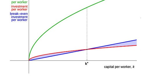
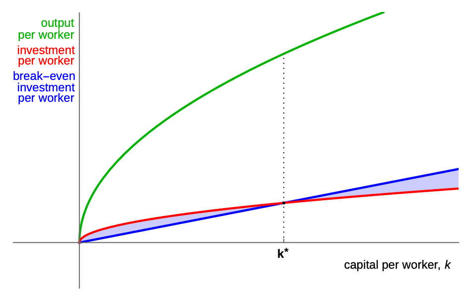
This motivates the Solow-Swan model, which can be represented graphically:
It makes three assumptions.
Firstly, output is determined by capital and labour, so output per worker is determined by capital per worker. This is the green line. Because there are decreasing returns to capital, it is a concave function.
Secondly, investment is a fixed share of output. This is the red line.
Thirdly, capital per worker naturally decreases over time, either because capital depreciates (from obsolescence or wear and tear) or because the workforce increases (from population growth). This is the blue line, called the “break-even” line because investment per worker must occur at the same rate for capital per worker to stay the same.
Consider what happens when capital per worker is below k*. That means investment per worker will be occurring faster than depreciation and population growth are, so over time, capital per worker will increase until we arrive at k*. Likewise, the converse will happen if we are above k*.
Thus there is an equilibrium of capital per worker at k*, with the corresponding output per worker marked by the dotted line. In the long run, GDP per capita will stay at the same level, so the Solow-Swan model cannot explain long-run economic growth!
However, it can account for changes in the short run. If the investment rate increases, this is represented by a higher red line. It’s clear that the new k* will be higher, and so correspondingly, the equilibrium GDP per capita will be higher too! In the period when the economy is transitioning to this new equilibrium, we will see economic growth! Of course, it is not possible to keep on doing this, because eventually the share of output allocated to investment would reach 100%, which is obviously absurd.
Phrases like the short run are always a bit ambiguous in economics, and in the case of the Solow-Swan model, the “short-run” transition dynamics can last on the order of 20 years! This is the story which best explains why many European countries were able to grow so quickly after World War Two, because although lots of capital was destroyed, they were simply catching up to where their equilibrium was pre-war. It also helps explain the East Asian growth miracles, which involved an enormous amount of investment and capital accumulation1.
More broadly, it implies that countries with similar investment rates and population growth rates will arrive at the same steady state GDP per capita. In practice, it seems that these differences explain around two-thirds of the variation in global GDP per capita2. That means factor accumulation cannot account for all of the cross-country income differences, nor can it explain long-run economic growth.
What can?
Endogenous growth
Productivity.
If your production processes keep getting better and can make more and more stuff with the same amount of capital and labour, then your living standard will rise! This is where the frontier of research on growth economics is today, trying to explain how and why productivity varies.
Productivity includes both ideas (improvements in technology) and institutions (more efficient resource allocation). Without doing a full review of the literature, I want to highlight a few trends in the former bucket! In particular, I want to show just how important the fall in the marginal cost of key resources has been.
One is the fall in energy prices, which enabled the Industrial Revolution to occur3!
Another is the fall in the price of computation, which catalysed the Digital Revolution!
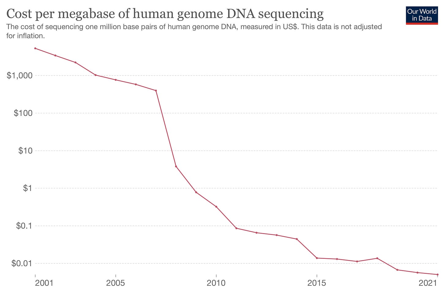
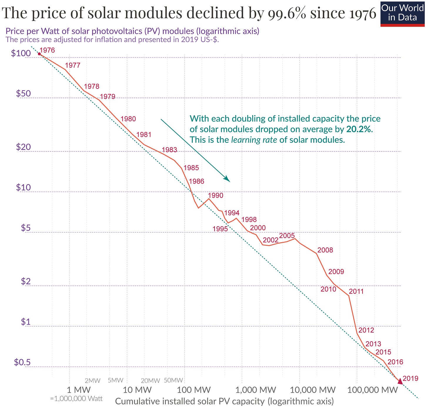
In fact, we are living through some of the most exciting declines in cost curves right now:
To the extent to which forecasting the future is possible, one of the best predictors is looking at the cost curves of key technologies: what happens when the cost of atoms, bits and cells all go to zero?


