


Damn Near Everything Is Endogenous
Let’s debunk a few monetary myths!

(h/t u/Integralds for the title)
Once again, money has caused a bit of a kerfuffle in econtwitter!


Given how prevalent these disputes over monetary theory and practice are, let’s settle this for once and for all. This post is an account of three things:
What money is
How money creation happens
How the monetary plumbing works.
If you came for the first tweet, see sections 1 and 2! If you came for the second tweet, see section 3!
What is money?
Money is an IOU
We don’t need money is an autarkic economy where no trades and transactions occur. Even in an exchange economy, we can barter goods for other goods without money. But barter sucks, because it relies on a double coincidence of wants. Both parties need something the other has. If that doesn’t occur, if that good is wanted at a different time or if that good is indivisible and in the wrong proportions, we’re screwed.
If I’m out with friends and forget to bring my wallet, they’ll cover for me. So a natural solution is to use IOUs. But debt only works if everyone can keep track of everyone else’s debts and trusts everyone to pay up. If we are a small group with thick-tie relationships, that’s alright. And many historical societies have functioned on the basis of debt and barter. But this doesn’t scale.
In our larger modern economies, we mostly trade across a network of thin-tie interactions. This means a personalised IOU is not reliable. Instead, we need a standardised one that keeps its value over time (so people will hold on to it), that can be used to measure the value of goods (so it is convenient in transactions) and that is widely accepted as an IOU (so you can execute most trades with it).
These three functions (store of value, unit of account and medium of exchange) are the canonical features of the social institution that is money. And by acting as a substitute for the societal memory of reciprocal financial obligations, money allows thin-tie exchange relationships to flourish easily.
Money is narrow and broad
Just like any IOU, money is a financial asset for the bearer. It represents a claim on something else in the economy. And correspondingly, it must be a financial liability for the person who issued it. In the modern economy, there are two sorts of money issued by two different people.
Narrow money, often termed the monetary base, is issued by central banks. It consists of electronic reserves and physical currency. When commercial banks make deposits at the central bank, they get reserves added to their central bank accounts. This money is a financial asset for the commercial bank and a financial liability for the central bank. Likewise, physical currency is a financial asset for the bearer and a financial liability for the central bank. In both cases, these IOUs are claims on the central bank - as such, they are seen as risk-free assets for households, firms and commercial banks.
By contrast, broad money is the money created by commercial banks and it represents the majority of money in the economy. Most people don’t want to hold all their IOUs in the form of notes and coins. This is because they are cumbersome and inconvenient to store, and they don’t earn any interest. As such, they put their physical currency into banks. In exchange for these assets, they get assets in return: namely, commercial bank deposits. Meanwhile, the commercial bank has created a new liability which they owe, in return for receiving an asset.
Deposits are the majority of broad money. But the majority of deposits aren’t created by people handing over currency. Rather, the very act of loan creation produces new deposits. When a bank makes a loan, they increase the deposits in someone’s accounts. This simultaneously creates a liability for the bank i.e. the reserves, as well as an asset for the bank i.e. the loan. In the same fashion, the borrower gains an asset i.e. the reserves, as well as a liability i.e. the loan. This is how banks can create money via lending.
How is money creation constrained?
Money is not a widow’s cruse
The story so far may sound a bit magical. How can banks money out of thin air? Are there any limits? As Hyman Minsky put it, “anyone can create money; the problem lies in getting it accepted”. And so the answer is that banks can create money because money is just a set of financial claims, and the limits on money creation are the limits on the extent to which they can make these claims.
Unfortunately, the usual mechanism that is given is not terribly accurate. The Economics 101 story goes like this. People make a real decision about how much to consume and save (read: “loanable funds” theory of interest determination). Their savings go to commercial banks, who hold some of that as central reserves but lend the rest of it out (read: “money multiplier” explanation of fractional reserve banking). In turn, that supply of money is mediated with the demand for money (read: “liquidity preference” theory of interest determination).
But as we’ve just seen, this is not how money creation works - banks do not need to rely on the depository behaviour of individual savers nor the central bank decisions regarding reserves to create a new loan. And it is damn confusing whether loanable funds or liquidity preference determine the interest rate - in fact, this just seems untenable. And yet the textbook narration is ultimately correct in that savings behaviour and central bank policy do constrain money creation. How does this happen?
Individual banks are not reserve constrained
Consider any individual bank. They will make loans as long as it is profitable for them to do so, taking into account considerations of risk as determined by their own judgement and that of prudential regulation. A bank is profitable as long as it earns more interest on assets than it pays on liabilities. Suppose a bank wants to increase its volume of loans. It can only do so by lowering the interest rate it charges. Borrowers will use the money to buy something from a seller, transferring their deposits to the bank of the seller. To match this transfer, the borrower’s bank must transfer corresponding reserves to the seller’s bank. Eventually the bank’s reserves will be exhausted.
But this doesn’t mean it is reserve-constrained as the “money multiplier” story might suggest. This is because there exists an interbank market for reserves, so it could borrow for more reserves from other banks. However, it is constrained by three things.
The interest rate of borrowing reserves from other banks i.e. the costs of operation.
The liquidity risk of relying on overnight interbank borrowing i.e. the potential inability to keep rolling over loans.
The credit risk from lending to customers i.e. the potential collapse in the revenue earned.
The underlying intuition behind these constraints is that money creation is about making IOUs and getting them accepted, and loans can only be formed out of assets. Since there are a limited amount of assets and given banks promise their money is backed by central bank money i.e. they commit to maintaining a 1:1 exchange rate on demand between the two, it is not possible to make unlimited amounts of money.
The banking system is maybe (?) reserve constrained
Okay, but if they’re borrowing on the interbank market then the banking system as a whole must be reserve constrained? Again, no. As it turns out, the banking sector as a whole is not reserve-constrained either, at least over some fixed period of time. Because central banks target a certain interest rate over some fixed time period (6 weeks for the Federal Reserve, European Central Bank and Bank of England), they will supply whatever quantity of reserves is necessary to meet bank demand for reserves at that price.
However, the behaviour of borrowers affects the degree to which the entire sector as a whole can create money. Think back to when someone borrows money. If borrowers use their new deposits to pay down debts, the net effect is that no new money is created. However, if it leads to spending on goods and services, this will bid up prices for those products and result in inflationary pressure. Central banks are generally mandated to keep inflation low and stable, so they will raise the prevailing interbank interest rate. This rise will result in fewer profitable loans, limiting money creation and allowing the central bank to meet its inflation target.
So let’s translate all of this back into 101 language. Firstly, it is true that broad money creation is endogenous to commercial bank behaviour over a 6 week interval. Think of this as liquidity preference where the money supply is perfectly interest elastic i.e. horizontal. Secondly, it is true that central banks have control over this across a longer time span, because they move their interest rate target over time i.e. the money multiplier story does convey the true claim that the central bank’s ability to control its own balance sheet can be used to affect broader measures of money. However, its implication that there is a stable relationship between the two is untrue. Thirdly, it is true that in the long run, loanable funds matter - while banks can create loans out of thin air, those depend on real assets which cannot be created out of thin air. And so the interest rate determined by loanable funds is still determinate in the long run - the way this is compatible with the other two parts of the story is because central banks try and make sure their interest rate target hits the implied interest rate of the loanable funds model!
How do central banks set policy?
Oh, wait a second. Just as the Economics 101 story was kind of a lie, I fudged something in what I’ve said so far too. And that’s because many central banks do not try to influence interbank interest rates by adjusting the money supply anymore. To understand this monetary plumbing, we need to go all the way back to before the financial crisis in 2008.
Targeting interest rates within a corridor
Consider the Federal Reserve1. Prior to the GFC, the Fed had three main tools.
The Fed set reserve requirements for depository institutions i.e. certain financial institutions had to hold a specific amount of money which couldn’t be lent out.
The Fed set the discount rate, which is the interest rate at which it lends to banks who provide collateral.
The Fed set the supply of reserves by engaging in open market operations.
At the time, banks could not earn returns on reserves, so they would try and keep that to its minimum requirements. That meant there was an active interbank market where banks lent reserves to each other overnight, if they needed reserves to meet these reserve requirements. This was the federal funds market. The prevailing market-determined interest rate in this federal funds market was called the federal funds rate, and since we know that interbank rates influence the volume of lending in the economy, the Fed set targets for this rate.
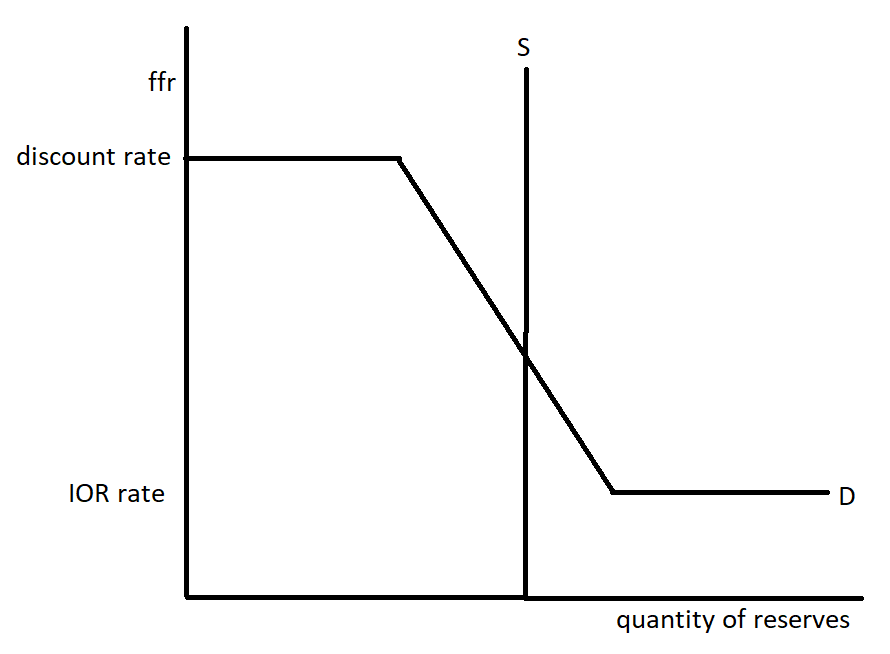
As with most demand curves, the demand curve for reserves is downwards-sloping. If it is cheaper to borrow, banks will demand more reserves. But there are two kinks and plateaus in this demand curve. To the left, no one is going to borrow at above the discount rate, since they could just borrow from the Fed. And to the right, everyone is going to borrow if there is no cost to borrowing, so it plateaus at 0.
As for the supply curve for reserves, this ws set by the Fed as a monopolistic supplier. It controlled the supply of reserves via open market operations. This is where it buys or sells government securities in exchange for reserves. Securities are just government debt, with Treasury bills being those that have a maturity of a year or less, Treasury notes being those between 2 to 10 years, Treasury bonds being those with 30-year maturities and Treasury Inflation-Protected Securities being 5, 10 and 30-year debts which are indexed to inflation.
These OMOs are done at the Trading Desk of the New York Fed. The desk buys a portfolio of Treasury securities which it holds, to ensure a baseline level of reserves. Then it adjusts this quantity via repurchase agreements with primary dealers. A repurchase agreement is a deal where one side sells an asset and promises to buy it back soon afterwards at a higher price - in effect, this is a way of doing collateralised lending i.e. lending where there is some sort of asset to back up the loan in case of default. It’s a bit like taking out a mortgage, where your house is used as collateral and can be seized by the bank if you fail to repay your mortgage on time. A primary dealer is a government securities dealer who has a trading relationship with the Fed.
So if the Fed wants to increase the supply of reserves, it will ask the desk to engage in repo agreements, by buying a Treasury security overnight and selling it back to the primary dealer the next day. Although this initially operates in the collateralised lending market rather than the uncollateralised lending market that is the federal funds market, primary dealers will deposit the money they receive at banks. Since they do operate within the federal funds market, this will increase the supply of reserves there. Via these OMOs, the Fed enacted monetary policy via this “corridor system”, where the intersection of the supply and demand curves determined the prevailing FFR. In many ways, this is quite similar to your usual liquidity preference diagram.
Targeting interest rates with a leaky floor
However, this changed during the financial crisis. The incredible volume of emergency bank lending from the Fed massively expanded the supply of reserves. According to Chairman Bernanke in “The Courage to Act”, this could have led “short-term interest rates to fall below our federal funds target and thereby cause us to lose control of monetary policy”. Although this was briefly offset by sterilisation i.e. contractionary OMOs where Treasury bonds were sold, this was not a long-term solution because the Fed did not have an indefinite amount of Treasuries to sell.
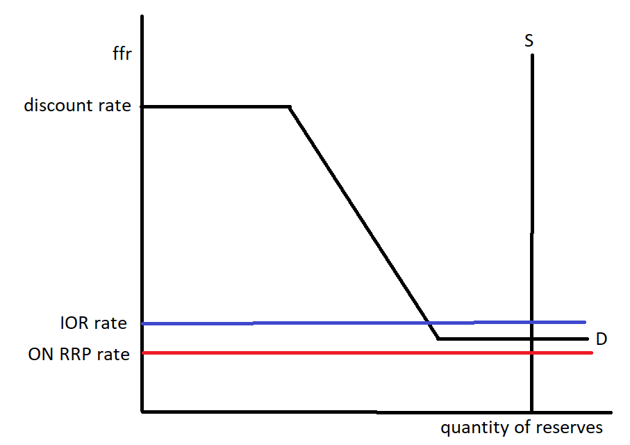
Consequently, the Fed introduced an additional tool: interest on reserves - this meant that it now paid banks on the reserves it held. Banks would have no incentive to lend at less than that, since they could earn those returns risk-free just by letting the reserves sit there. As such, the discount rate and IOR rate set a ceiling and a floor on the FFR. And since 2008, the supply of reserves is so ample that it intersects the demand curve at the IOR rate. This is the “floor system”, where the FFR is determined not within a corridor of values but by the level at which the floor is set, allowing the Fed control even with an oversaturation of reserves.
In practice, it’s a little more complicated than the description above. Firstly, there are actually three discount rates. The primary credit rate is the rate at which financially sound institutions can borrow. The secondary credit rate is slightly higher, and is for institutions which may be smaller and less sound. The seasonal credit rate even higher, and is for institutions which face seasonally-variant cash flows. And sometimes banks do borrow at a rate above all the discount rates, because there is a stigma associated with needing to borrow at the discount window from the Fed i.e. it signals that you are unable to get private counterparty banks to lend to you.
Secondly, there were two IOR rates: there is an interest rate paid on required reserves and an interest rate paid on excess reserves. However, this has been rendered redundant right now because the reserves requirement has been set to 0 since the covid-19 crisis, equalising the IORR and IOER. And in fact, this doesn’t act as an exact floor either, because not every financial institution in the federal funds market has access to IOR. So they could potentially be willing to lend at even below the IOR rate, pushing the FFR below this floor.
This is why the Fed introduced overnight reverse repurchase agreements to this broader set of institutions. These are the reverse of the repo agreements discussed previously, allowing financial institutions to deposit reserves overnight and receive Treasuries as collateral, with the Fed buying back the Treasuries the next day for slightly more than the reserves deposited i.e. in effect lending to the Fed at the ON RRP rate. In practice, the federal funds rate has been somewhere in between the IOR and the ON RRP rate since this introduction.
It is true that the implementation of this leaky floor has given the Fed a more direct way of controlling the FFR via simply adjusting the IOR and ON RRP rates instead of through OMOs, allowing for emergency lending not to cause the FFR to plummet. But this is not costless. In particular, the fact that the FFR is at or below the IOR is unhelpful, because it means that the creation of extra reserves does not necessarily increase bank lending. Instead, commercial banks may decide that they can hoard these reserves instead of using it for more bank loan creation. So it becomes easy for monetary policy to be too tight2. Not only does this neuter the effectiveness of monetary policy, it also reduces the volume of lending in the federal funds market - this is especially problematic, because it reduces the incentive to monitor interbank risks3.
Unconventional tools in unconventional times
So far, we’ve seen how the Fed can use reserve requirements, the discount rates, IOR rates, ON RRP rates and temporary OMOs via repo to influence the FFR. But beyond just changing the manner in which the FFR is determined through these tools, the Fed has also expanded its range of options since the GFC in three main ways.
Large-scale asset purchases of quantitative easing and credit easing.
Forward guidance and conditional commitment.
Emergency lending facilities and credit swap lines.
Large-scale asset purchases are similar in principle to OMOs as a form of monetary policy i.e. they involve the Fed buying up assets, raising their prices and lowering their yields. The result of this wealth effect and cheaper borrowing costs bolster economic activity. However, there are a few differences in practice. Firstly, this is done on a far larger scale than the usual OMOs - hence the name. Secondly, LSAPs involve a much wider range of assets - rather than just buying the usual government securities, the Fed also bought up longer-term government securities, mortgage-backed securities and corporate bonds. This means that the effect is expanded beyond the very short-run. Thirdly, there are different sorts of LSAPs. Quantitative easing is aimed at increasing the money supply, while credit easing is aimed at reducing long-term interest rates by specifically considering the composition of assets it is buying up.
For forward guidance and conditional commitment, these terms refer to “open mouth operations” conducted by the Fed i.e. the use of words as a tool of monetary policy. Because agents in the economy are forward-looking, the Fed’s words regarding what it plans to do and the conditions upon which it is going to engage in easing or tightening set expectations which affect their behaviour. In practice, the effectiveness of this sort of talk depends on its credibility. On the one end is Delphic forward guidance, where the Fed simply alludes to the likely state of the world in the future, as though it were the Oracle of Delphi. On the other end is Odyssean forward guidance, where the Fed binds itself to future policy actions conditional upon certain indicators, much as Odysseus bound himself to the mast of his ship.
A particularly profound level of commitment is the Fed’s recent shift in its policy regime. In the past, it had looked at its dual mandate of 2% inflation and full employment as one where the Fed targeted 2% inflation every year. If it missed the target, it would still be targeting 2% inflation the next year. The problem with this is that if the target is missed again and again (as it has been since 2008), people’s inflationary expectations will fall and so actual inflation will too, resulting in further misses. The new regime of average inflation targeting ensures that the Fed is committed to making up for shortfalls, such that inflation averages 2% over time. Suppose there is a demand-side shock that pushes down output and inflation - the advantage of this approach is that even when nominal interest rates are near 0, the credible expectations of future inflation will reduce longer-run real interest rates too, making monetary policy more potent.
And finally, emergency lending facilities are essentially programs the Fed can set up to support specific lending and funding markets in “unusual and exigent circumstances” under Section 13(3) of the Federal Reserve Act. Since the passing of the Dodd-Frank Act in 2010, the Fed’s ability to engage in these programs has been vastly limited, only to be available with the consent of the Treasury and only for programs with “broad-based eligibility”. These facilities ensure that key financial markets which the broader financial ecosystem depends upon do not fail. For example, the market for Treasury securities is important, because the interest rates on Treasuries act as a baseline benchmark for many other interest rates. When the market is illiquid in its market liquidity i.e. it is difficult to buy and sell those assets, this means the transactions necessary for financial markets to accurately be used for risk management and investment is disrupted. Now in the case of Treasuries, OMOs are already used for this purpose - but there are plenty of other asset markets where it is necessary for the Fed to set up ad hoc lending liquidity and credit facilities. The Fed also engages in emergency liquidity provision at an international scale via dollar swap lines - in effect, the Fed lets foreign central banks exchange their currency for dollars. This is important due to the global role the dollar has, as it ensures other central banks can support dollar-denominated markets in their own countries.
In the aftermath of the 2008 crisis, the Fed engaged in all of these policies. It engaged in three rounds of LSAPs (2008-2010, 2010-2011 and 2012-2014)4. It also conducted the Maturity Extension Program - commonly known as Operation Twist, this kept the size of the Fed balance sheet the same but changed the composition of Treasuries to those with longer maturities. In effect, this was a way of committing to a lower-for-longer approach, in conjunction with the language of its public statements5. And of course, it deployed a whole host of emergency 13(3) facilities. In the covid-19 crisis, the Fed once again engaged in all of these policies6.
How does it all fit together?
So let’s reminds ourselves of what this all looks like together. Monetary policy in the US involves a leaky floor to set the federal funds rate and the use of unconventional tools to affect monetary conditions more broadly. This interbank rate affects the profitability and volume of lending in the money market, with the broad money supply being decided on endogenously by commercial banks in the period where the federal funds rate target is fixed. Over time, the Federal Reserve adjusts its instruments to affect the federal funds rate and hence the supply of broad money, ensuring it meets its dual mandate of low and stable inflation as well as maximum employment. And in the long run, the interest rate necessary to meet these goals are implied by the real consumption-savings decisions made by the population at large. Loanable funds, the money multiplier and liquidity preference all have their place - but as monetary policy evolves, the simplified stories we tell should also evolve. And that means being clearer about 1. how money endogeneity resolves itself (note: IS-LM is about how we reconcile loanable funds with liquidity preference) and 2. how the Federal Reserve controls broad money i.e. why money multiplier is an acceptable approximation over some time spans but not others.